Artificial Neural Network (ANN)
Introduction to Artificial Neural Network (ANN):
An Artificial Neural Network (ANN) used in deep learning, consists of different layers connected to each other and it is a computational model that is inspired by the way biological neural networks in the human brain process information. It learns from huge volumes of data and uses complex algorithms to train a neural net. Artificial Neural Networks have generated a lot of excitement in Machine Learning research and industry, thanks to many breakthrough results in speech recognition, computer vision and text processing.
Let’s Understand Single Neuron:
The neuron is the basic unit of computation in a neural network and it often called a node or unit. It receives input from some other nodes or from an external source and computes an output. Each input has an associated weight (w), which is assigned based on its relative importance to other inputs. The node applies a function f (defined below) to the weighted sum of its inputs as shown in the figure below.
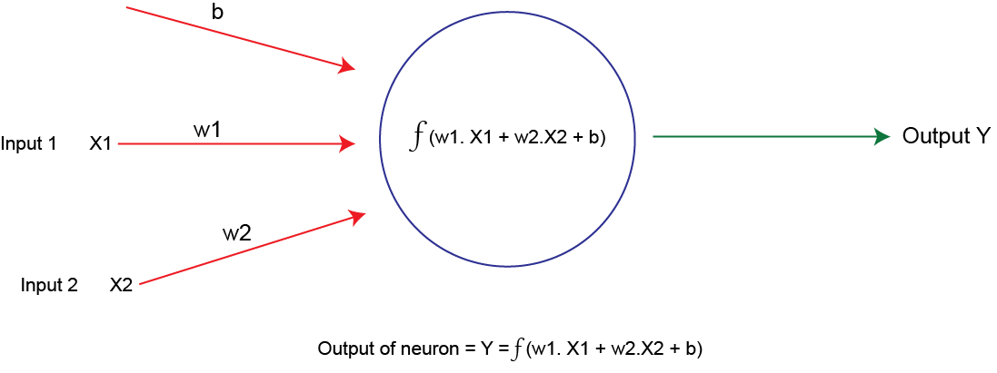
Figure 1: Figure of a single neuron
The above network takes numerical inputs like X1, X2 and has weights w1 and w2 associated with those inputs. There is another input 1 with weight b associated with it. It is called Bias (b). The output Y from the neuron is computed as shown in the figure 1. The function f is non-linear and is called the activation function. Activation function is used to introduce non-linearity into the output of a neuron. Every activation function takes a single number and performs a certain fixed mathematical operation on it. There are several types of activation functions we use.
## Sigmoid Function: Sigmoid function also known as logistic function or logistic curve and it is look like “S” shape. The equation of sigmoid function is given below:
e1f(x)= L/(1+ e^(-k(x-x_0)) )
In the sigmoid function equation “e” stands for Euler’s number, “x0” stands for the x-value of the sigmoid midpoint, L stands for the curve’s maximum value and k stands for the steepness of the curve. The main reason why we use sigmoid function is because it exists between 0 to 1. Therefore, it is especially used for models where we have to predict the probability as an output. Since probability of anything exists only between the range of 0 and 1, sigmoid is the right choice. The function is differentiable. That means, we can find the slope of the sigmoid curve at any two points. The function is monotonic but function’s derivative is not. The logistic sigmoid function can cause a neural network to get stuck at the training time. The softmax function is a more generalized logistic activation function, which is used for multiclass classification. Figure of sigmoid function given below.
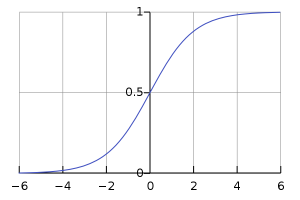
Figure 2: Figure of sigmoid function
Threshold Function:
A threshold function is a Boolean function that determines whether a value equality of its inputs exceeded a certain threshold. A device that implements such logic is known as a threshold gate. It’s also known as Step function or Heaviside step function. The equation of threshold function is given below:
e2
Using second equation, Let n Boolean inputs be x1,x2…xn. f is a function that decides whether w1x1 + w2x2 + … + wnxn = t where t is a real number called the threshold and w1, w2, .. wn are real-numbered weights. A threshold function on n Boolean inputs x1, x2, …, xn is then a Boolean function that decides whether w1x1 + w2x2 + … + wnxn ≥ t. Figure of threshold function given below.
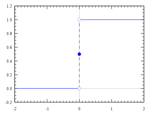
Figure 3: Figure of threshold function
Rectifier Linear Unit Activation Function (ReLU):
ReLU is an activation function that defined as the positive part of its argument. The ReLU is the most used activation function in the world right now. Since, it is used in almost all the convolutional neural networks or deep learning. Its equation is:
e3
In the equation x the is input to a neuron. This is also known as a ramp function. Rectified linear units find applications in computer vision and speech recognition using deep neural nets. The function and its derivative both are monotonic. But the issue is that all the negative values become zero immediately which decreases the ability of the model to fit or train from the data properly. That means any negative input given to the ReLU activation function turns the value into zero immediately in the graph, which in turns affects the resulting graph by not mapping the negative values appropriately. Figure of threshold function given below.
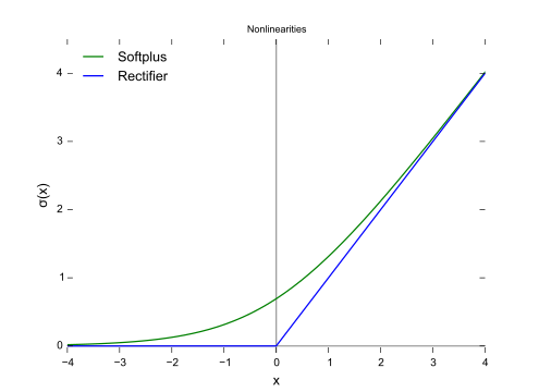
Figure 4: Figure of ReLU activation function
Tanh or Hyperbolic Tangent Activation Function: Tanh is also like logistic sigmoid but better. The range of the tanh function is from -1 to 1. Tanh is also sigmoidal s-shaped. Equation of Tanh is:
e4
The advantage is that the negative inputs will be mapped strongly negative and the zero inputs will be mapped near zero in the tanh graph. The function is differentiable. The function is monotonic while its derivative is not monotonic. The tanh function is mainly used classification between two classes. Both tanh and logistic sigmoid activation functions are used in feed-forward nets.
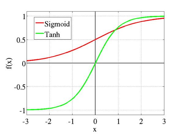
Figure 5: Figure of Tanh activation function with Sigmoid
Let’s try to understand Bias:
A Bias neuron allows a classifier to shift the decision boundary left or right. In an algebraic term, the bias neuron allows a classifier to translate its decision boundary. To translation is to “move every point a constant distance in a specified direction”. A bias unit is an “extra” neuron added to each pre-output layer that stores the value of 1. Bias units aren’t connected to any previous layer and in this sense don’t represent a true “activity”.
Take a look at the following illustration:
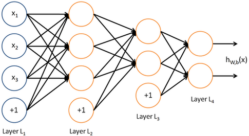
Figure 6: Figure of Bias in layer
The bias units are characterized by the text “+1”. We can see, a bias unit is just appended to the end of the input and each hidden layer, and isn’t influenced by the values in the previous layer. In other words, these neurons don’t have any incoming connections.
Bias units still have outgoing connections and they can contribute to the output of the ANN. Let’s call the outgoing weights of the bias units w_b. Now, let’s look at a really simple neural network that just has one input and one connection:
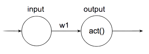
Figure 7: Figure of Bias
Let’s say act() our activation function is just f(x) = x, or the identity function. In such case, our ANN would represent a line because the output is just the weight (m) times the input (x).
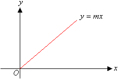
Figure 8: Figure of Bias
When we change our weight w1, we will change the gradient of the function to make it steeper or flatter.
So, we know that our function output = w · input (y = mx) needs to have this constant term added to it. In other words, we can say output = w · input + w_b, where w_b is our constant term c. When we use neural networks, though, or do any multi-variable learning, our computations will be done through Linear Algebra and matrix arithmetic eg. dot-product, multiplication. This can also be seen graphically in the ANN. There should be a matching number of weights and activities for a weighted sum to occur. Because of this, we need to “add” an extra input term so that we can add a constant term with it. Since, one multiplied by any value is that value, we just “insert” an extra value of 1 at every layer. This is called the bias unit.
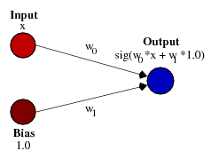
Figure 9: Figure of Bias in layer
From this diagram, you can see that we have now added the bias term and hence the weight w_b will be added to the weighted sum, and fed through activation function as a constant value. This constant term, also called the “intercept term”, shifts the activation function to the left or to the right. It will also be the output when the input is zero. Here is a diagram of how different weights will transform the activation function (sigmoid in this case) by scaling it up/down.
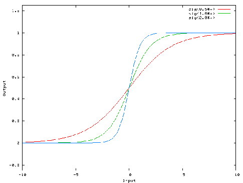
Figure 10: Figure of Bias in sign waves
But now, by adding the bias unit, we the possibility of translating the activation function exists:
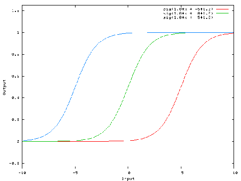
Figure 11: Figure of Bias in sign waves
Going back to the linear regression example, if w_b = 1, then we will add bias · w_b= 1 · w_b = w_b to the activation function. In the example with the line, we can create a non-zero y-intercept:
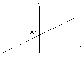
Figure 12: Figure of Bias
I’m sure you can imagine infinite scenarios where the line of best fit does not go through the origin or even come near it. Bias units are important with neural networks in the same way.
How do Neural Network Work:
Consider that we have some parameters about the property. We have area in square feet, number of bedrooms, distance from the city and the age of the property and all of those four are going to comprise as the input layer. Now of course they are probably way more parameters that define the price of a property. It is a very basic form of a neural network and it only has an input layer and output layer. It has no hidden layers and our output layer is the price that we are predicting. So here inputs variables would just be weighted up by the synopses and then output would be calculated. Basically the price would be calculated and get a price. And for instance the price could be calculated as simple as the weighted sum of all of the inputs.
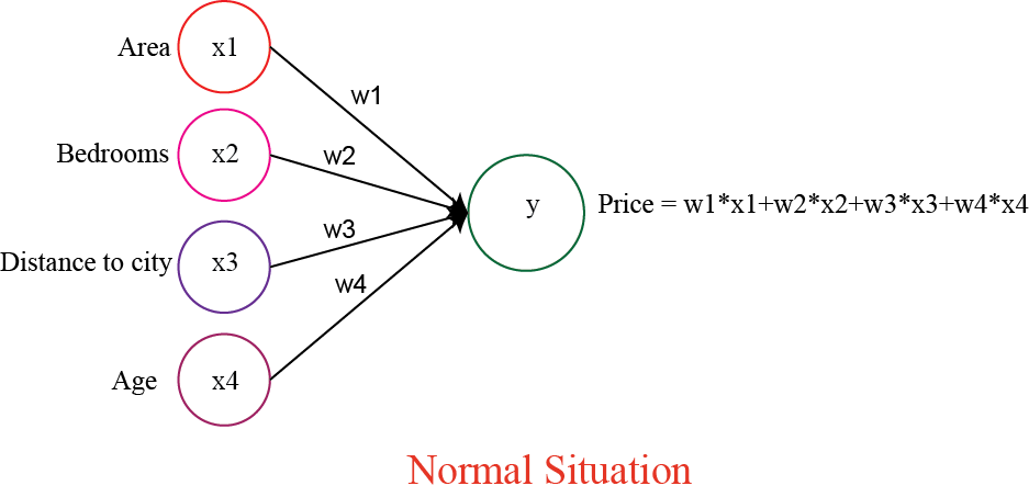
Figure 13: Figure of Neural Network without hidden layer.
Now let’s make our network a little more complex. Here, and in all neural network diagrams, the layer on the far left is the input layer, and the layer on the far right is the output layer (the network’s prediction/answer). Any number of layers in between these two are known as hidden layers. The more the number of layers, the more nuanced the decision-making can get.
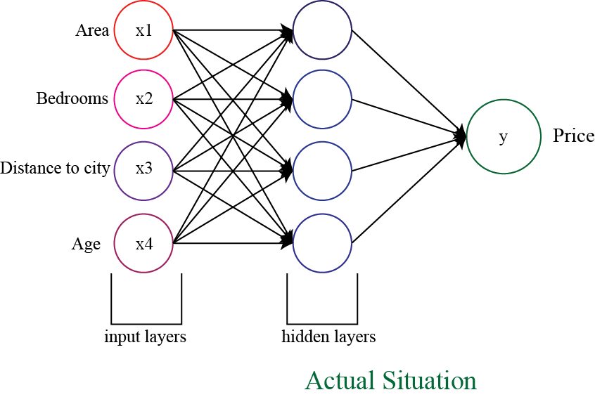
Figure 14: Figure of Neural Network with hidden layer.
Now with the hidden layers artificial neural network follow some steps for work. All the steps are given below.
Figure 15: Figure of Steps of how Neural Network work.
The networks often go by different names: deep feedforward networks, feedforward neural networks, or multi-layer perceptron’s (MLP). Let’s talk about feed forward neural network.
Feedforward Neural Network:
The feedforward neural network was the first and simplest type of artificial neural network devised. It contains multiple neurons (nodes) arranged in layers. Nodes from adjacent layers have connections or edges between them. All these connections have weights associated with them.
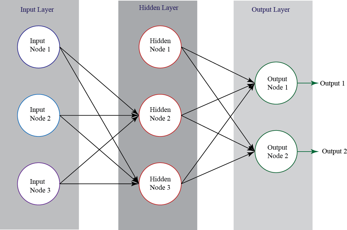
Figure 16: Figure of Feed Forward Neural Network.
A feedforward neural network can consist of three types of nodes:
1. Input Nodes:
The Input nodes provide information from the outside world to the network and are together referred to as the “Input Layer”. No computation is performed in any of the Input nodes. They just pass on the information to the hidden nodes.
2. Hidden Nodes:
The Hidden nodes have no direct connection with the outside world (hence the name “hidden”). They perform computations and transfer information from the input nodes to the output nodes. A collection of hidden nodes forms a “Hidden Layer”. While a feedforward network will only have a single input layer and a single output layer, it can have zero or multiple Hidden Layers.
3. Output Nodes:
The Output nodes are collectively referred to as the “Output Layer” and are responsible for computations and transferring information from the network to the outside world.
In a feedforward network, the information moves in only one direction which is forward direction from the input nodes, through the hidden nodes (if any) and to the output nodes. There are no cycles or loops in the network. This property of feed forward networks is different from Recurrent Neural Networks in which the connections between the nodes form a cycle.
Two examples of feedforward networks are given below:
1. Single Layer Perceptron – Single Layer Perceptron is the simplest feedforward neural network and does not contain any hidden layer.
2. Multi-Layer Perceptron – A Multi-Layer Perceptron has one or more hidden layers. We will only discuss Multi-Layer Perceptrons below since they are more useful than Single Layer Perceptions for practical applications today.
A Multi-Layer Perceptron (MLP) contains one or more hidden layers (apart from one input and one output layer). While a single layer perceptron can only learn linear functions, a multi-layer perceptron can also learn non linear functions.
Figure 17 shows a multi-layer perceptron with a single hidden layer. Note that all connections have weights associated with them, but only three weights (w0, w1, w2) are shown in the figure.
Input Layer:
The Input layer has three nodes. The Bias node has a value of 1. The other two nodes take X1 and X2 as external inputs (which are numerical values depending upon the input dataset). As discussed above, no computation is performed in the Input layer, so the outputs from nodes in the Input layer are 1, X1 and X2 respectively, which are fed into the Hidden Layer.
Hidden Layer:
The Hidden layer also has three nodes with the Bias node having an output of 1. The output of the other two nodes in the Hidden layer depends on the outputs from the Input layer (1, X1, X2) as well as the weights associated with the connections (edges). Figure 17 shows the output calculation for one of the hidden nodes (highlighted). Similarly, the output from other hidden node can be calculated. Remember that f refers to the activation function. These outputs are then fed to the nodes in the Output layer.
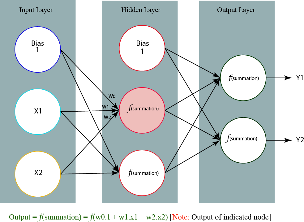
Figure 17: Figure of a Multi-Layer perceptron with a single hidden layer.
Output Layer:
The Output layer has two nodes which take inputs from the Hidden layer and perform similar computations as shown for the highlighted hidden node. The values calculated (Y1 and Y2) as a result of these computations act as outputs of the Multi-Layer Perceptron.
Given a set of features X = (x1, x2, …) and a target y, a Multi-Layer Perceptron can learn the relationship between the features and the target, for either classification or regression.
Let us take an example to understand Multi-Layer Perceptrons better. Suppose we have the following student marks dataset:
| Hours Studied | Mid Term Marks | Final Term Result |
|---|---|---|
| 35 | 67 | 1(Pass) |
| 12 | 75 | 0(Fail) |
| 16 | 89 | 1(Pass) |
| 45 | 56 | 1(Pass) |
| 10 | 90 | 0(Fail) |
The two input columns show the number of hours the student has studied and the mid-term marks obtained by the student. The Final Result column can have two values 1 or 0 indicating whether the student passed in the final term. For example, we can see that if the student studied 35 hours and had obtained 67 marks in the mid-term, he or she ended up passing the final term. Now, suppose, we want to predict whether a student studying 25 hours and having 70 marks in the mid term will pass the final term.
| Hours Studied | Mid Term Marks | Final Term Result |
|---|---|---|
| 25 | 70 | ? |
This is a binary classification problem where a multi-layer perceptron can learn from the given examples (training data) and make an informed prediction given a new data point. We will see below how a multi-layer perceptron learns such relationships.
Training Multi-Layer Perceptron:
The process by which a Multi-Layer Perceptron learns is called the Backpropagation algorithm. I would recommend reading this Quora answer (quoted below) which URL given below where explains Backpropagation clearly.
Backward Propagation of Errors, often abbreviated as BackProp is one of the several ways in which an artificial neural network (ANN) can be trained. It is a supervised training scheme, which means, it learns from labeled training data (there is a supervisor, to guide its learning).
To put in simple terms, BackProp is like “learning from mistakes“. The supervisor corrects the ANN whenever it makes mistakes.
An ANN consists of nodes in different layers; input layer, intermediate hidden layer(s) and the output layer. The connections between nodes of adjacent layers have “weights” associated with them. The goal of learning is to assign correct weights for these edges. Given an input vector, these weights determine what the output vector is. In supervised learning, the training set is labeled. This means, for some given inputs, we know the desired/expected output (label).
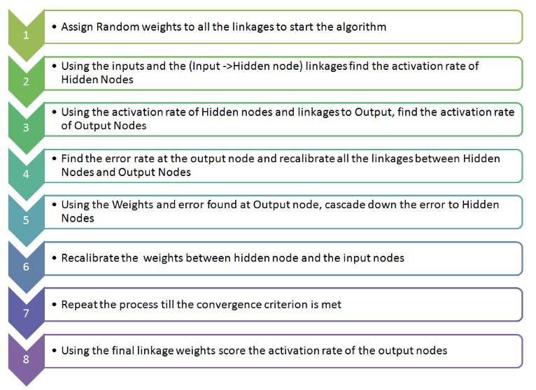
BackProp Algorithm: Initially all the edge weights are randomly assigned. For every input in the training dataset, the ANN is activated and its output is observed. This output is compared with the desired output that we already know, and the error is “propagated” back to the previous layer. This error is noted and the weights are “adjusted” accordingly. This process is repeated until the output error is below a predetermined threshold.
Once the above algorithm terminates, we have a “learned” ANN which, we consider is ready to work with “new” inputs. This ANN is said to have learned from several examples (labeled data) and from its mistakes (error propagation).
Now that we have an idea of how Backpropagation works, let us come back to our student-marks dataset shown above. The Multi Layer Perceptron shown in Figure 18 (adapted from Sebastian Raschka’s excellent visual explanation of the backpropagation algorithm) has two nodes in the input layer (apart from the Bias node) which take the inputs ‘Hours Studied’ and ‘Mid Term Marks’. It also has a hidden layer with two nodes (apart from the Bias node). The output layer has two nodes as well the upper node outputs the probability of ‘Pass’ while the lower node outputs the probability of ‘Fail’.
In classification tasks, we generally use a Softmax function as the Activation Function in the Output layer of the Multi-Layer Perceptron to ensure that the outputs are probabilities and they add up to 1. The Softmax function takes a vector of arbitrary real-valued scores and squashes it to a vector of values between zero and one that sum to one. So, in this case,
Probability (Pass) + Probability (Fail) = 1
Step 1: Forward Propagation
All weights in the network are randomly assigned. Let us consider the hidden layer node marked V in Figure 18 below. Assume the weights of the connections from the inputs to that node are w1, w2 and w3 (as shown).
The network then takes the first training example as input (we know that for inputs 35 and 67, the probability of Pass is 1).
• Input to the network = [35, 67]
• Desired output from the network (target) = [1, 0]
Then output V from the node in consideration can be calculated as below (f is an activation function such as sigmoid):
V = f (1*w1 + 35*w2 + 67*w3)
Similarly, outputs from the other node in the hidden layer is also calculated. The outputs of the two nodes in the hidden layer act as inputs to the two nodes in the output layer. This enables us to calculate output probabilities from the two nodes in output layer.
Suppose the output probabilities from the two nodes in the output layer are 0.4 and 0.6 respectively (since the weights are randomly assigned, outputs will also be random). We can see that the calculated probabilities (0.4 and 0.6) are very far from the desired probabilities (1 and 0 respectively), hence the network in Figure 18 is said to have an ‘Incorrect Output’.

Figure 18: Figure of Forward Propagation
Step 2: Back Propagation and Weight Updating
We calculate the total error at the output nodes and propagate these errors back through the network using Backpropagation to calculate the gradients. Then we use an optimization method such as Gradient Descent to ‘adjust’ all weights in the network with an aim of reducing the error at the output layer. This is shown in the Figure 19 below (ignore the mathematical equations in the figure for now). Suppose that the new weights associated with the node in consideration are w4, w5 and w6 (after Backpropagation and adjusting weights).
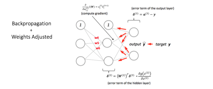
Figure 19: Figure of Back Propagation and Weight Updating
If we now input the same example to the network again, the network should perform better than before since the weights have now been adjusted to minimize the error in prediction. As shown in Figure 20, the errors at the output nodes now reduce to [0.2, -0.2] as compared to [0.6, -0.4] earlier. This means that our network has learnt to correctly classify our first training example.

Figure 20: Figure of correct output.
We repeat this process with all other training examples in our dataset. Then, our network is said to have learnt those examples.
If we now want to predict whether a student studying 25 hours and having 70 marks in the mid-term will pass the final term, we go through the forward propagation step and find the output probabilities for Pass and Fail.
I have avoided mathematical equations and explanation of concepts such as ‘Gradient Descent’ here and have rather tried to develop an intuition for the algorithm. For a more mathematically involved discussion of the Backpropagation algorithm, refer to this link.
Three Basic Questions for ANN:
Question 1: What is the correlation between the time consumed by the algorithm and the volume of data (compared to traditional models like logistic)?
Answer: As mentioned above, for each observation ANN does multiple re-calibrations for each linkage weights. Hence, the time taken by the algorithm rises much faster than other traditional algorithm for the same increase in data volume.
Question 2: In what situation does the algorithm fits best?
Answer: ANN is rarely used for predictive modelling. The reason being that Artificial Neural Networks (ANN) usually tries to over-fit the relationship. ANN is generally used in cases where what has happened in past is repeated almost exactly in same way. For example, say we are playing the game of Black Jack against a computer. An intelligent opponent based on ANN would be a very good opponent in this case (assuming they can manage to keep the computation time low). With time ANN will train itself for all possible cases of card flow. And given that we are not shuffling cards with a dealer, ANN will be able to memorize every single call. Hence, it is a kind of machine learning technique which has enormous memory. But it does not work well in case where scoring population is significantly different compared to training sample. For instance, if I plan to target customer for a campaign using their past response by an ANN. I will probably be using a wrong technique as it might have over-fitted the relationship between the response and other predictors. For same reason, it works very well in cases of image recognition and voice recognition.
Question 3: What makes ANN a very strong model when it comes down to memorization?
Answer: Artificial Neural Networks (ANN) have many different coefficients, which it can optimize. Hence, it can handle much more variability as compared to traditional models.
