Break Down Lenet-1

2019, Oct 26    

Introduction:

Currently, we all curious about image processing work. Deep learning plays an important role in image classification tasks. In deep learning, a convolutional neural network (CNN) which is famous for image processing tasks. CNN build on layers, and they are convolution, pooling, flatten and fully connected layer. With the help of these layers to improve the CNN, various sorts of architecture buildup by researchers. Now I will discuss an architecture known as LeNet-1 architecture. In the discussion, I will breakdown every step, how an input image shape turns into various shapes. I hope my simple discussion help all of you to understand CNN.

Prerequisite:

You have to understand how convolution, pooling and fully connected layer work. Otherwise, you will not understand.

How to calculate shape:

At first, we need to know how to calculate shape. Its important and help to understand and breakdown all the architecture of CNN. When we apply convolution, pooling to the image, the calculation of the shape helps to understand what will be the output after applying convolution and pooling. The equation which generally use to calculate the shape given below. It’s applicable when height and the width of the image are the same.

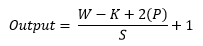
Here, W is the height or width of the image. K is the height or width of the single filter or kernel. P is the number of padding. S is the number of pixels shift over the input matrix.

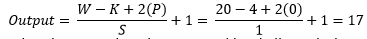
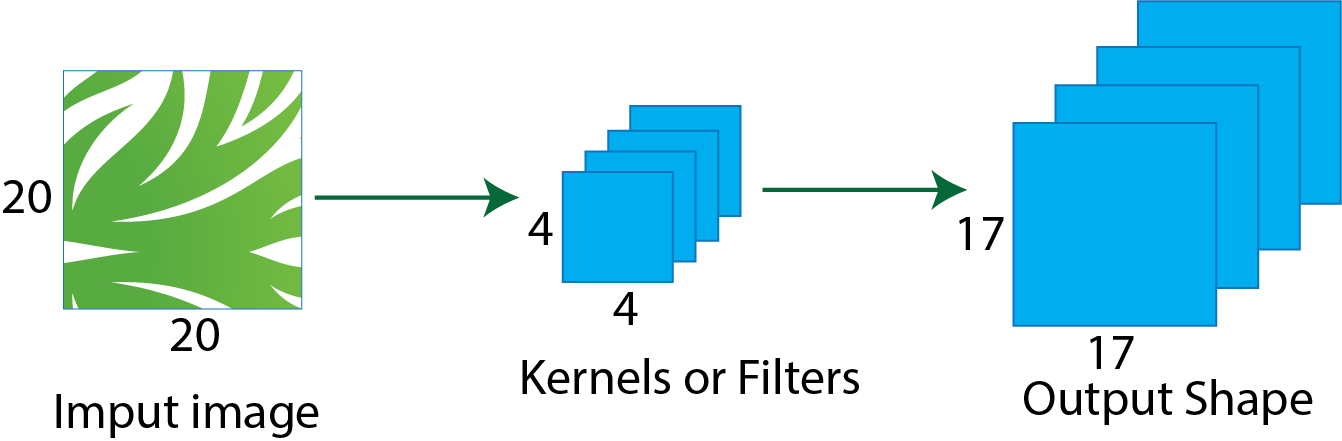
An example image presented below. Where, the size of the input image is 20X20, size of single filter 4X4 and the size of the output shape 17X17, which is the result. So from the image we consider the value of W is 20, the value of K is 4, the value of P is 0 as there is no extra padding in the image and the value of the stride is 1 (consider). After applying these values in the equation, the output is 17.

So, from the above equation, the output shape is 17X17, and it’s similar to the image presented below.

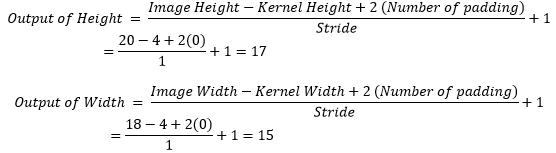
If the height and width of the image are not equal, then the equation will be the same, but the elements of the equation must different based on the height and width. Need to calculate output shape for the height and width separately. The equation to calculate the output shape of the height given below.

The equation to calculate the output shape of the width given below.

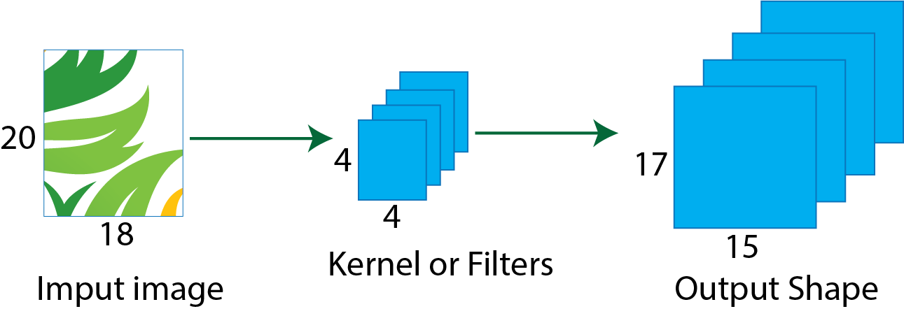
An example image presented below. Where, the size of the input image is 20X18, size of single filter 4X4 and the size of the output shape 17X15, which is the result. So from the image we consider the value of the height of the input image is 20, the width of the input image is 18, the value of the height of the kernel is 4, the value of the width of the kernel is 4, number of padding is 0 as there is no extra padding in the image and the value of the stride is 1 (consider). After applying these values in the separate equation for height and width, the output shape is 17X15 (height is 17 and width is 15), and it’s similar to the image presented below.

Now, Its time to break down LeNet-1 architecture. The common image of the LeNet-1 architecture presented below. The LeNet-1 architecture is a first simple architecture for the convolutional neural network. It’s easy to understand and implement.

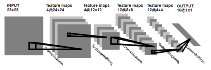
The specification of the LeNet-1 presented below layerwise. Input shape of the image is 28X28. Four 24X24 feature maps in the convolutional layer by using four 5X5 kernels or filters. Four 12X12 feature maps in the average pooling layer by using four 2X2 kernels or filters. Twelve 8X8 feature maps in the convolution layer by using twelve 5X5 kernels or filters. Twelve 4X4 feature maps in the average pooling layer by using twelve 2X2 kernels or filters. Directly fully connected to the output layers of 10 units.

Now, try to understand visually how every step works in the LeNet-1 architecture.

First Step:

In the first step, try to understand the input image to the first convolution layer. The process of this step presented below in the picture.

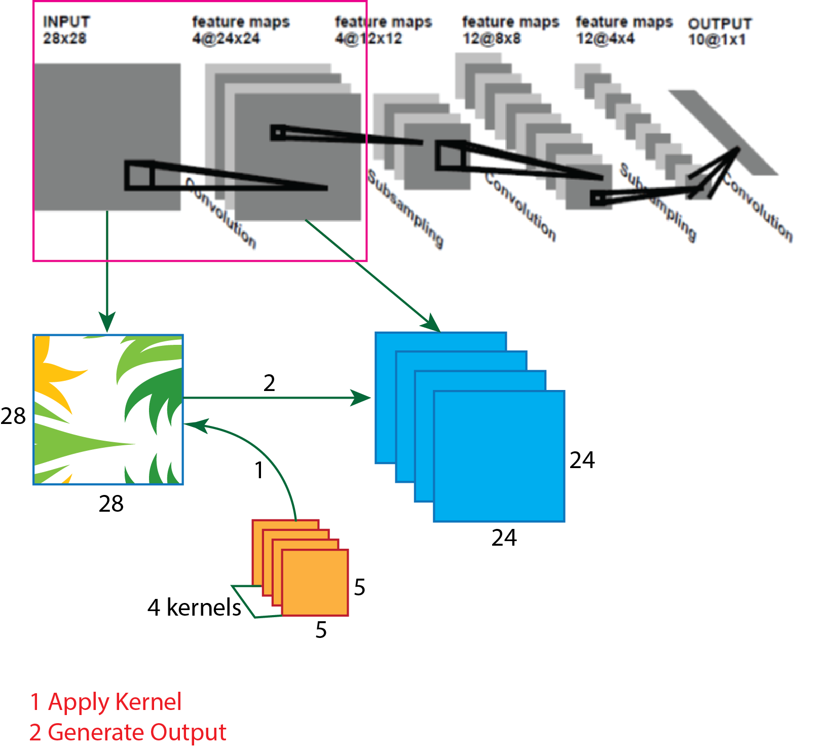
To generate the first convolution layer from the input image, four 5X5 size kernels used. Now we use equation which helps to calculate output shape. The parameters for calculation given below:

1. Input size 28X28X1 (assume 2D image) (W=28).
2. A total number of kernels 4.
3. Single kernel size 5X5 (K=5)
4. Number of padding 0 (P=0)
5. Stride 1 (S=1)

Now insert all the values in the equation.

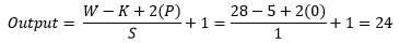
So, after the calculation, the result is as same as the image, and the output shape of the first convolution layer is 24X24X4.

Second Step:

In the second step, try to understand the first convolution layer to first average pooling layer. The process of this step presented below in the picture.

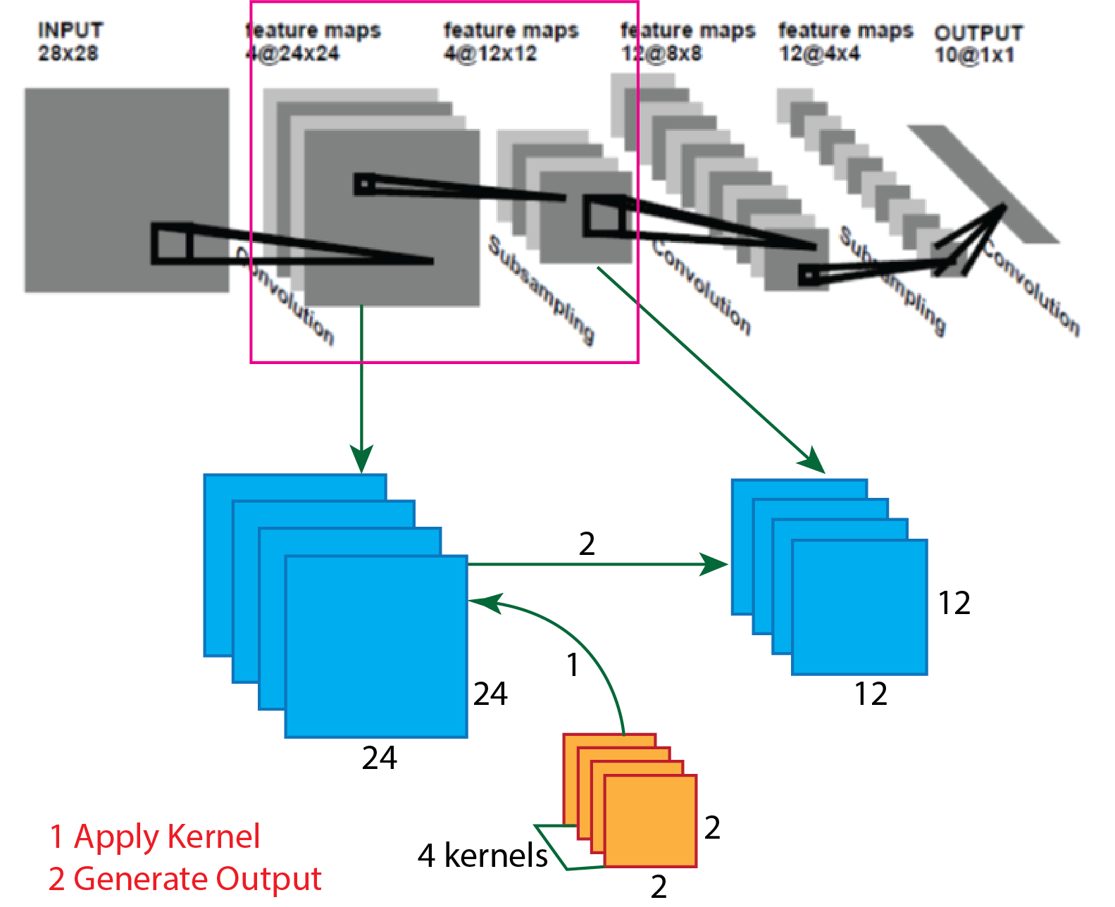
To the generate the first average pooling layer from the first convolution layer, four 2X2 size kernels used. Now we use equation which helps to calculate output shape. The parameters for the calculation given below:

1. Input size 24X24X4 (W=24).
2. A total number of kernels 4.
3. Single kernel size 2X2 (K=2)
4. Number of padding 0 (P=0)
5. Stride 2 (S=2)

Now insert all the values in the equation.

So, after the calculation, the result is as same as the image, and the output shape of the first average pooling layer is 12X12X4.

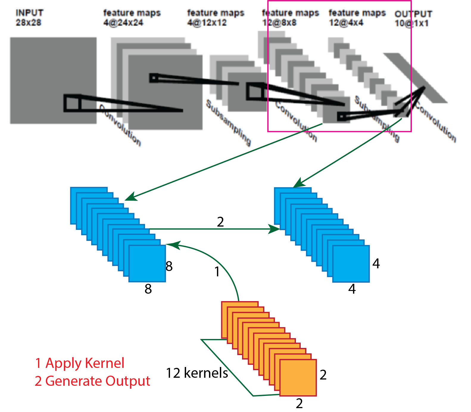
Third Step:

In the third step, try to understand the first average pooling layer to the second convolution layer. The process of this step presented below in the picture.

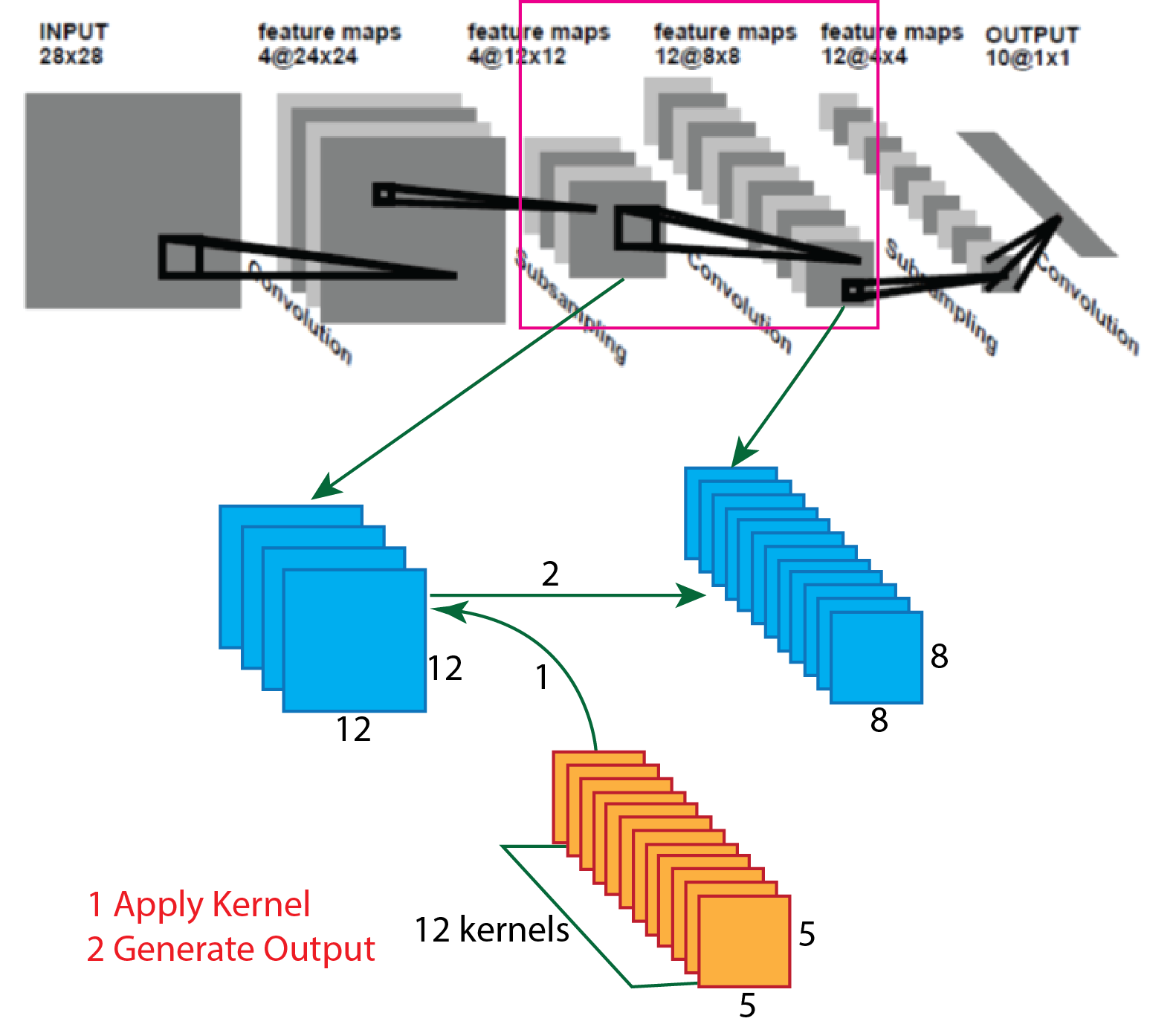
To the generate the second convolution layer from the first average pooling layer, twelve 5X5 size kernels used. Now we use equation which helps to calculate output shape. The parameters for calculation given below:

1. Input size 12X12X4 (W=12).
2. A total number of kernels 12.
3. Single kernel size 5X5 (K=5)
4. Number of padding 0 (P=0)
5. Stride 1 (S=1)

Now insert all the values in the equation.

Fourth Step:

In the fourth step, try to understand the second convolution layer to the second average pooling layer. The process of this step presented below in the picture.

To generate the second average pooling layer from the second convolution layer, twelve 2X2 size kernels used. Now we use equation which helps to calculate output shape. The parameters for the calculation given below:

1. Input size 8X8X12 (W=8).
2. A total number of kernels 12.
3. Single kernel size 2X2 (K=2)
4. Number of padding 0 (P=0)
5. Stride 2 (S=2)

Now insert all the values in the equation.

So, after the calculation, the result is as same as the image, and the output shape of the first average pooling layer is 4X4X12.

Fifth Step:

In the fifth step, try to understand the second average pooling layer to flatten layer and connected to the output layer. The process of this step presented below in the picture.

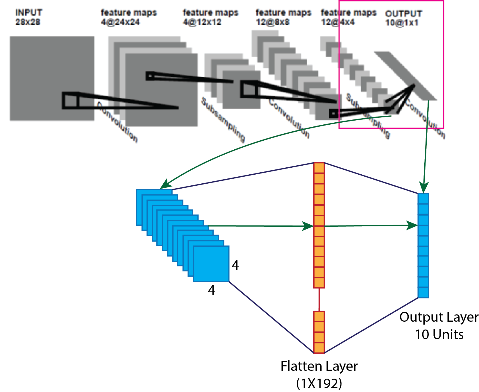
To connect directly average pooling layer to output layer, first, need to build flatten layer from the average pooling layer and then connect to the output layer. The shape of the flatten layer is 1X192. All the neurons or the units of the flatten layer fully connected to the neurons or units of the output layer.

By following this way, LeNet-1 architecture buildup. In the architecture tanh used as an activation function.

If this post helpfull for you than share it…